Introduction to Feedforward Neural Network - Comprehensive Tutorial

Table of Contents

Artificial Neural Networks (ANNs)

The introduction of Artificial Neural Networks (ANNs) into machine learning has been a game changer as they have proven to be effective tools for pattern recognition, classification and predictive modeling. Over many years, many neural network techniques has been developed, but Feedforward Neural Network (FNN) is the most common technique that works with machines and deep learning. In this tutorial, we will explore the key concepts behind feedforward neural networks, their architecture, functioning, applications and how they function. This tutorial will provide a comprehensive understanding on the essential techniques of this machine learning model.

Introduction to Feedforward Neural Networks

An Artificial Neural Network (ANN) is a computer system which resembles the network of neurons in the brain, which can imitate the biological activity of a human body by understanding how human brain process information. It comprises layers that consist of interconnected units known as neurons. Artificial Neural networks (ANN) can be used for a variety of applications including: classification, regression and more complex applications like pattern recognition.

A Feedforward Neural Network (FNN) is regarded as one of the simplest and most widely used Neural Network architecture applied in machine learning tasks. It consists of multiple layers of neurons in which the flow of information is unidirectional, that starts from the input layer and then gets to the output layer by way of other layers in the process of communication or a transmission of a signal. Because of its unidirectional flow it is known as Feedforward.

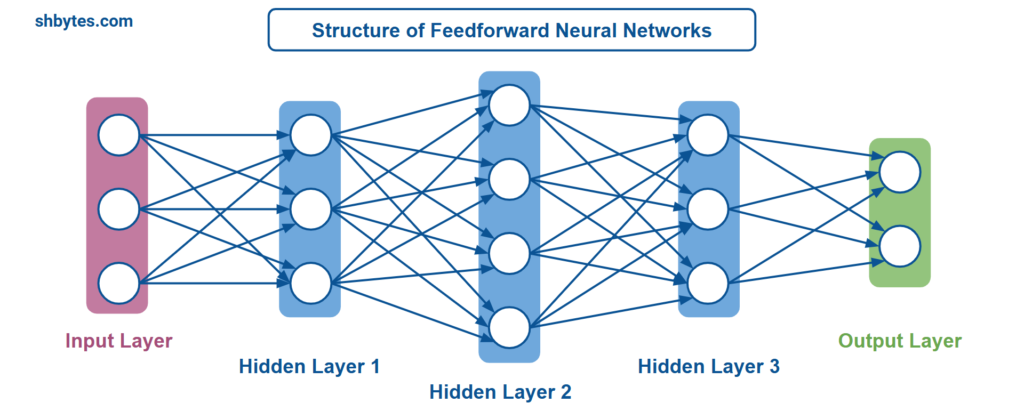
Structure of Feedforward Neural Networks

A Feedforward Neural Network (FNN) can be classified into different layers: input, output and hidden layer.

Neurons or Nodes: Neurons are the basic computational units of a neural network. Each neuron takes an input, applies a weight and bias to it, along with an activation function, and forwards the result to the next layer.

Input Layer – The purpose of this layer is to receive the input data. This input layer consists of many neurons, where each neuron represents a feature of the input data.
Hidden Layers – There are many middle-ware layers in between the the input and output layers. Because we do not directly interact with these layers, that is why they are called hidden layers. These layers also contains neurons which are used to perform calculations based on inputs received from the previous layer. Output of one layer becomes the input for another layer. The number of hidden layers and neurons in each layer can be changed depending on the complexity of the problem.
Output Layer – This is the final layer, which gives the prediction or classification result of the network. In general, the output layer contains one neuron for each class in a classification problem or one neuron for each output in regression problems. So, the number of neurons required in this layer depends on the number of classes in a classification problem or number of outputs in regression problem.

**Structure of Feedforward Neural Networks**

Key Components of Feedforward Neural Network

Weights and Biases

Each connection between neurons has an associated weight, which determines the strength of that connection. The weight signifies how much influence the input will have on the output of the neuron.
In addition to weights, each neuron has a bias. The bias allows the model to make adjustments to the output regardless of the input, helping the neural network learn more complex patterns. Bias is added to the weighted sum of the inputs before applying the activation function.

Activation Function

An activation function is used to transform the weighted sum of inputs to the output of the neuron. The activation function introduce non-linearity into the network and determines if a neuron will “fire” (i.e., activate) or not based on the input it receives. This enables the system to learn and model complex data patterns. Commonly used activation functions include:

Sigmoid – This function outputs a value between 0 and 1. This is commonly used in binary classification.
- $σ(x) = \frac{1}{1 + e^{-x}}$
ReLU (Rectified Linear Unit) – If the input is positive, then this function outputs it directly; otherwise, zero is returned as an output.
- $ReLU(x)=max(0,x)$
Tanh (Hyperbolic Tangent) – This function outputs values between -1 and 1. This function is used when a network needs outputs with a broader range than sigmoid.
- $tanh(x) = \frac{e^{x} – e^{-x}}{e^{x} + e^{-x}}$
Softmax – This function is used in the output layer for multi-class classification. This function produces a probability distribution over the classes.

Forward Propagation

Forward propagation refers to the process of passing input data through the network to obtain an output. For each layer in the network, the following formula is used to compute the output.

Multiply the input by the weights.
Add the bias term.
Apply the activation function.

Mathematically, for a neuron $i$ in a layer $l$:

$z_{i}^{(l)} = \sum_{j}^{}w_{ij}^{(l)}x_{j}^{(l-1)} + b_{i}^{(l)}$

$a_{i}^{(l)} = activation (z_{i}^{(l)})$

Where:

$w_{ij}^{(l)}$ is the weight from neuron $j$ in layer $l−1$ to neuron $i$ in layer $l$.
$x_{j}^{(l-1)}$ is the output from neuron $j$ in the previous layer $l−1$.
$b_{i}^{(l)}$ is the bias term for neuron $i$.
$activation(⋅)$ is the activation function applied to the weighted sum.

Training Feedforward Neural Networks

The idea of training a neural network is to tune the weights and biases in such a way that the difference between the predicted output from the network and the actual value (or label) gets minimized. This process is usually called supervised learning, which essentially includes two major steps:

Forward Pass – The input flows through the network, and an output is computed as described above.
Backpropagation – After computation of output, the predicted output is compared with true target value using a proper loss function. The error is then allowed to flow backward in a network by adjusting weights and biases so that it minimizes the error.

Loss Function

The loss function measures the difference between the network’s predicted output and the true target values. Loss function helps the model learn by minimizing this difference during training. Common loss functions include:

Mean Squared Error (MSE) Loss – Measures the average squared difference between predicted values and the actual values. This loss function is mainly used for regression tasks.
Cross-Entropy Loss (Log Loss) – Measures the difference between two probability distributions – the true distribution (actual labels) and the predicted distribution. This loss function is mainly used for classification tasks.
Categorical Cross-Entropy Loss – Generalizes binary cross-entropy to multi-class problems.

Read article Loss Functions in Machine Learning: Unlocking the Secrets to Model Optimization

Backpropagation

During the backpropagation the error is allowed to pass backward in the network to update the weights and biases. The calculates the gradient of the loss function with respect to each weight and bias. This gradient is used to adjust the weights in the direction that reduces the error.

The gradient of the loss function $L$ with respect to a weight $w$ is calculated using the chain rule.

$\frac{\partial L}{\partial w} = \frac{\partial L}{\partial a} . \frac{\partial a}{\partial z} . \frac{\partial z}{\partial w}$

Where:

$\frac{\partial L}{\partial a}$ is the derivative of the loss with respect to the activation output.
$\frac{\partial a}{\partial z}$ is the derivative of the activation function with respect to the weighted sum.
$\frac{\partial z}{\partial w}$ is the derivative of the weighted sum with respect to the weight.

Gradient Descent

Gradient Descent is an optimization algorithm used to minimize the loss function in machine learning models, particularly in deep learning. It helps to calculate the gradient of the loss function for each weight and bias in neural networks that minimize the error between the model’s predictions and the actual data. Once the gradients are calculated, the weights and biases are adjusted using gradient descent optimization algorithm.

$w := w – \eta . \frac{\partial L}{\partial w}$

where, $\eta$ is the learning rate, which controls how much to adjust the weights during each update.

Types of Gradient Descent

Batch Gradient Descent – Uses the entire dataset to compute the gradient and update the parameters at each step.
Stochastic Gradient Descent (SGD) – Uses only one randomly chosen data point to compute the gradient and update the parameters in each iteration.
Mini-Batch Gradient Descent – A compromise between batch and stochastic gradient descent. It uses a small random subset (mini-batch) of the dataset to compute the gradient and update the parameters in each iteration.

Hyperparameters of Feedforward Neural Networks

Performance of feedforward neural networks is influenced by several hyperparameters that are fixed before training.

Number of layers – Defines the depth of the network. More layers can help the network learn complex representations.
Number of neurons per layer – Affects the network capacity in capturing patterns; too few layers may lead to under-fitting, while too many layers can result in over-fitting.
Learning Rate – This controls the step size for updating weights. If too high, convergence may not happen, while too low will result in slow training.
Batch Size – The number of samples to include in one iteration of gradient descent.
Epochs – How many times the whole dataset passes through this network during training.

Challenges and Considerations

Overfitting – If the network is too complex or trained for too many epochs, it might memorize the training data it has seen instead of generalizing to new training data. Regularization techniques like dropout, L2 regularization, or early stop can help avoid over-fitting.
Vanishing Gradient Problem – The gradient in deep networks can become very small in the back-propagation process, thereby making it hard for the network to learn. Most of the time, one would prefer using ReLU over sigmoid and tanh for activation functions to avoid this problem.
Computational Cost – Generally, training large neural networks can be rather computationally expensive, taking considerable time and resources. Mini-batch gradient descent or stochastic gradient descent (SGD) methods are used to reduce computation.

Example Program: A Simple Feedforward Neural Network in Python (Using Keras)

import tensorflow as tf
from tensorflow.keras.models import Sequential
from tensorflow.keras.layers import Dense
from tensorflow.keras.optimizers import Adam
import numpy as np

# Example input data
x = [[0.1, 0.2, 0.3], [0.2, 0.4, 0.5], [0.5, 0.5, 0.5], [0.6, 0.7, 0.8]]

# Ensure the input is a Tensor or Numpy array
x = np.array(x)

# Define the model
model = Sequential()

# Input layer with 3 features
model.add(Dense(15, input_dim=3, activation='relu'))  # Hidden layer with 15 neurons
model.add(Dense(1, activation='sigmoid'))   # Output layer for binary classification

# Compile the model
model.compile(loss='binary_crossentropy', optimizer=Adam(), metrics=['accuracy'])

# Fit the model (assuming y is correctly defined)
y = np.array([0, 0, 1, 1])

# Train the model
model.fit(x, y, epochs=5, batch_size=1)  # epoch - number of iterations for dataset

# Evaluate the model
loss, accuracy = model.evaluate(x, y)
print(f'Accuracy: {accuracy}')

This example program demonstrates the building, training, and evaluating a neural network model using TensorFlow and Keras. We have defined x as input dataset, converted to NumPy array to feed into the model. The model architecture is defined using the Sequential API. We added two layers – first layer with 15 neurons and ReLU activation mechanism and second layer as output layer with sigmoid activation mechanism. We train the model with epoch=5 for 5 iterations. Finally calculate the loss and accuracy of the model.

Output – Example Program – Feedforward Neural Network using Keras

Epoch 1/5
4/4 ━━━━━━━━━━━━━━━━━━━━ 1s 4ms/step - accuracy: 0.7333 - loss: 0.6826  
Epoch 2/5
4/4 ━━━━━━━━━━━━━━━━━━━━ 0s 2ms/step - accuracy: 0.4333 - loss: 0.7460
Epoch 3/5
4/4 ━━━━━━━━━━━━━━━━━━━━ 0s 1ms/step - accuracy: 0.4333 - loss: 0.7744     
Epoch 4/5
4/4 ━━━━━━━━━━━━━━━━━━━━ 0s 2ms/step - accuracy: 0.3667 - loss: 0.7892
Epoch 5/5
4/4 ━━━━━━━━━━━━━━━━━━━━ 0s 1ms/step - accuracy: 0.4333 - loss: 0.7354
1/1 ━━━━━━━━━━━━━━━━━━━━ 0s 140ms/step - accuracy: 0.5000 - loss: 0.7335
Accuracy: 0.5, Loss: 0.7335233688354492

Conclusion

Feedforward neural networks are the foundation of neural network architecture. To work with machine learning and deep learning algorithms, one should have good understanding of neural network structures, how they work with forward propagation and backpropagation and how to use them to train models. In this way, when we understand the very foundations of neural networks, we can go ahead and build complex neural network architectures for several applications like image recognition, natural language processing, and more.

Code snippets and programs related to Feedforward Neural Network, can be accessed from GitHub Repository. This GitHub repository all contains programs related to other topics in LLM (Large Language Models) tutorial.

Introduction to Feedforward Neural Network – Comprehensive Tutorial