
Loss Functions in Machine Learning
A loss function is a mathematical function, which is also called a cost function or objective function. Loss function in machine learning is used to measure the accuracy of model’s predictions matching it with the actual target values. The purpose of machine learning model training is to improve the accuracy of the model’s prediction by minimizing the value of loss function. In this explanation, we’ll cover the importance of loss functions, their role in machine learning model training, and the various types of loss functions used for different tasks.
Importance of Loss Functions in Machine Learning
In machine learning, a model is used to make predictions or generate language response based on the given input data. However, these predictions or language responses are not completely perfect. The loss function in machine leaning measures the difference between the network’s predicted output and the true target values. Basically, it quantifies the discrepancy between the predicted values and the actual values, by providing an error or loss value. Loss functions in machine learning helps the model to learn by minimizing this discrepancy during model training.
- During training the machine learning models adjusts their parameters like weights and biases to minimize the value of loss function. Minimizing this loss function value will help ML models to improve their predictions.
- The goal is to minimize the loss function during training through optimization techniques like Gradient Descent.
Key Concepts of Loss Functions
- Predicted value: The value that the model predicts for a given input.
- Actual value: The actual value or label for the given input in the training dataset.
- Error: The difference between the predicted value and the actual value. The loss function calculates this error across all data points.
The formula for a general loss function is: $L(\widehat{y}, y) = loss(y, \widehat{y})$, where
- $y$ is the true value.
- $\widehat{y}$ is the predicted value.
- $L(\widehat{y}, y)$ represents the loss between the true and predicted values.
Types of Loss Functions in Machine Learning
The choice of loss function depends on the type of machine learning task. Loss functions in machine learning are categorized in three categories:
- Loss Function for Regression
- Loss Function for Classification
- Loss Function for Specialized Tasks
Loss Function for Regression
In regression tasks, the goal is to predict a continuous output. For example, predicting house prices, stock prices, or temperature values.
Mean Squared Error (MSE)
The Mean Squared Error (MSE) is one of the most common loss function for regression problems. It calculates the square of the difference between the predicted and true values, then takes the average over all data points.
MSE = $\frac{1}{n} \sum_{i=1}^{n}(y_{i} – \widehat{y}_{i})^{2}$
Where, $n$ is the number of data points. $y_{i}$ is the true value for the $i$-th data point. $\widehat{y}_{i}$ is the predicted value for the $i$-th data point.
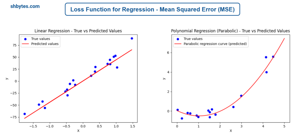
Example Program – Linear Regression using Mean Squared Error (MSE)
# Import necessary libraries
import numpy as np
from sklearn.model_selection import train_test_split
from sklearn.linear_model import LinearRegression
from sklearn.metrics import mean_squared_error
from sklearn.datasets import make_regression

# 1. Create a synthetic dataset
X, y = make_regression(n_samples=100, n_features=1, noise=10, random_state=42)

# 2. Split the dataset into training and testing sets
X_train, X_test, y_train, y_test = train_test_split(X, y, test_size=0.2, random_state=42)

# 3. Initialize the model
model = LinearRegression()

# 4. Train the model using the training data
model.fit(X_train, y_train)

# 5. Make predictions on the test data
y_pred = model.predict(X_test)

# 6. Calculate the Mean Squared Error (MSE)
mse = mean_squared_error(y_test, y_pred)

# Print the MSE
print(f"Mean Squared Error (MSE): {mse}")

# Output => Mean Squared Error (MSE): 104.20222653187027
Example Program – Polynomial Regression using Mean Squared Error (MSE)
# Import necessary libraries
import numpy as np
from sklearn.model_selection import train_test_split
from sklearn.preprocessing import PolynomialFeatures
from sklearn.linear_model import LinearRegression
from sklearn.metrics import mean_squared_error

# 1. Create a synthetic dataset that follows a parabolic relationship
# Generate X values (random data)
np.random.seed(42)
X = np.sort(5 * np.random.rand(80, 1), axis=0)  # 80 samples between 0 and 5

# Create the parabolic target values (y = ax^2 + bx + c + noise)
y = 0.5 * X**2 - X + np.random.randn(80, 1) * 0.5  # Parabolic relationship with some noise

# 2. Split the dataset into training and testing sets
X_train, X_test, y_train, y_test = train_test_split(X, y, test_size=0.2, random_state=42)

# 3. Initialize the PolynomialFeatures class with degree 2 for a parabolic fit
poly = PolynomialFeatures(degree=2)

# 4. Transform the input data to include polynomial features (X^2)
X_train_poly = poly.fit_transform(X_train)
X_test_poly = poly.transform(X_test)

# 5. Train a linear regression model using the transformed polynomial features
model = LinearRegression()
model.fit(X_train_poly, y_train)

# 6. Make predictions on the test data
y_pred = model.predict(X_test_poly)

# 7. Calculate the Mean Squared Error (MSE)
mse = mean_squared_error(y_test, y_pred)
print(f"Mean Squared Error (MSE): {mse}")

# Output => Mean Squared Error (MSE): 0.1701467841288596
Mean Absolute Error (MAE)
Mean Absolute Error (MAE) is a common evaluation metric used to assess the performance of regression models. It measures the average magnitude of the absolute differences between predicted and actual values, without considering their direction (i.e., it doesn’t distinguish between overestimation or underestimation). In simple terms, MAE tells us the average “absolute” difference between the predicted and actual values, making it an easy-to-understand metric for model performance.
MAE = $\frac{1}{n} \sum_{i=1}^{n}|y_{i} – \widehat{y}_{i}|$
Where, $n$ is the number of data points. $y_{i}$ is the true value for the $i$-th data point. $\widehat{y}_{i}$ is the predicted value for the $i$-th data point.
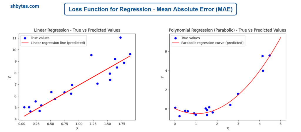
Example Program – Linear Regression using Mean Absolute Error (MAE)
# Import necessary libraries
import numpy as np
from sklearn.model_selection import train_test_split
from sklearn.linear_model import LinearRegression
from sklearn.metrics import mean_absolute_error

# 1. Create a synthetic linear dataset
np.random.seed(42)

# Generate X values (random data)
X = 2 * np.random.rand(100, 1)  # 100 samples between 0 and 2

# Create the linear target values (y = 4 + 3x + noise)
y = 4 + 3 * X + np.random.randn(100, 1)  # Linear relationship with some noise

# 2. Split the dataset into training and testing sets
X_train, X_test, y_train, y_test = train_test_split(X, y, test_size=0.2, random_state=42)

# 3. Initialize and train the Linear Regression model
model = LinearRegression()
model.fit(X_train, y_train)

# 4. Make predictions on the test data
y_pred = model.predict(X_test)

# 5. Calculate the Mean Absolute Error (MAE)
mae = mean_absolute_error(y_test, y_pred)
print(f"Mean Absolute Error (MAE): {mae}")

# Output => Mean Absolute Error (MAE): 0.5913425779189777
Example Program – Polynomial Regression using Mean Absolute Error (MAE)
# Import necessary libraries
import numpy as np
from sklearn.model_selection import train_test_split
from sklearn.preprocessing import PolynomialFeatures
from sklearn.linear_model import LinearRegression
from sklearn.metrics import mean_absolute_error

# 1. Create a synthetic dataset that follows a parabolic relationship
# Generate X values (random data)
np.random.seed(42)
X = np.sort(5 * np.random.rand(80, 1), axis=0)  # 80 samples between 0 and 5

# Create the parabolic target values (y = ax^2 + bx + c + noise)
y = 0.5 * X**2 - X + np.random.randn(80, 1) * 0.5  # Parabolic relationship with some noise

# 2. Split the dataset into training and testing sets
X_train, X_test, y_train, y_test = train_test_split(X, y, test_size=0.2, random_state=42)

# 3. Initialize the PolynomialFeatures class with degree 2 for a parabolic fit
poly = PolynomialFeatures(degree=2)

# 4. Transform the input data to include polynomial features (X^2)
X_train_poly = poly.fit_transform(X_train)
X_test_poly = poly.transform(X_test)

# 5. Train a linear regression model using the transformed polynomial features
model = LinearRegression()
model.fit(X_train_poly, y_train)

# 6. Make predictions on the test data
y_pred = model.predict(X_test_poly)

# 7. Calculate the Mean Absolute Error (MAE)
mae = mean_absolute_error(y_test, y_pred)
print(f"Mean Absolute Error (MAE): {mae}")

# Output => Mean Absolute Error (MAE): 0.3120968863393948
Huber Loss
Huber Loss is a loss function for regression problems that is less sensitive (linear) for large errors than Mean Squared Error (MSE) but more sensitive (quadratic) for small errors than Mean Absolute Error (MAE). It combines the strengths of both MSE and MAE, making it robust and efficient in various scenarios.
Huber Loss = $\left\{ \begin{array}{cl} \frac{1}{2} (y_{i} – \widehat{y}_{i})^{2} &\text{ for} |y_{i} – \widehat{y}_{i}| \le \delta \\ \delta |y_{i} – \widehat{y}_{i}| – \frac{1}{2}\delta^{2} &\text{ for} |y_{i} – \widehat{y}_{i}| \gt \delta\end{array} \right.$
Where $\delta$ is a threshold parameter.
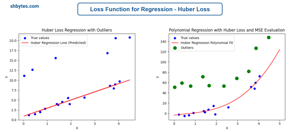
Example Program – Linear Function Huber Loss with Mean Absolute Error
import numpy as np
from sklearn.linear_model import HuberRegressor
from sklearn.model_selection import train_test_split
from sklearn.metrics import mean_absolute_error

# 1. Generate synthetic data (with a linear relationship + some noise)
np.random.seed(42)

# Generate X values (100 samples)
X = np.sort(5 * np.random.rand(100, 1), axis=0)

# Generate the target values (y = 2 * X + 1 with added noise)
y = 2 * X + 1 + np.random.randn(100, 1)  # Linear relationship with Gaussian noise

# 2. Introduce outliers to the data
y[::10] = y[::10] + 10  # Every 10th value has a large outlier

# 3. Split the dataset into training and testing sets
X_train, X_test, y_train, y_test = train_test_split(X, y, test_size=0.2, random_state=42)

# 4. Initialize and train the Huber Regressor model
model = HuberRegressor()
model.fit(X_train, y_train)

# 5. Make predictions using the trained model
y_pred = model.predict(X_test)

# 6. Calculate the Mean Absolute Error (MAE) to evaluate the model
mae = mean_absolute_error(y_test, y_pred)
print(f"Mean Absolute Error (MAE): {mae}")

# Output => Mean Absolute Error (MAE): 3.483117828288826
Example Program – Polynomial Function Huber Loss with Mean Squared Error
import numpy as np
from sklearn.preprocessing import PolynomialFeatures
from sklearn.linear_model import HuberRegressor
from sklearn.model_selection import train_test_split
from sklearn.metrics import mean_squared_error

# 1. Generate synthetic polynomial data (with some noise and outliers)
np.random.seed(42)

# Generate 100 samples (X)
X = np.sort(5 * np.random.rand(100, 1), axis=0)

# Generate polynomial target values (y = X^3 + Gaussian noise)
y = X**3 + np.random.randn(100, 1) * 10  # Cubic relationship with noise

# 2. Introduce some outliers
y[::10] = y[::10] + 50  # Every 10th value has a large outlier

# 3. Split the dataset into training and testing sets
X_train, X_test, y_train, y_test = train_test_split(X, y, test_size=0.2, random_state=42)

# 4. Transform the input data into polynomial features (degree 3 for cubic relationship)
poly = PolynomialFeatures(degree=3)
X_poly_train = poly.fit_transform(X_train)
X_poly_test = poly.transform(X_test)

# 5. Initialize and train the Huber Regressor model (which uses Huber Loss)
model = HuberRegressor()
model.fit(X_poly_train, y_train)

# 6. Make predictions using the trained model
y_pred = model.predict(X_poly_test)

# 7. Calculate Mean Squared Error (MSE) for the predictions
mse = mean_squared_error(y_test, y_pred)
print(f"Mean Squared Error (MSE): {mse}")

# Output => Mean Squared Error (MSE): 1041.9669985250653
Loss Functions for Classification
Classification tasks involve predicting categorical labels, such as whether an email is spam or not. The loss function for classification typically measures how well the predicted probability distributions match the true class distributions.
Cross-Entropy Loss (Log Loss)
The Cross-Entropy Loss, also known as Log Loss, is the most commonly used loss function for classification tasks. It measures the distance between the true label distribution and the predicted label distribution. For binary classification, it compares the predicted probabilities of the classes with the true binary labels.
Binary Cross-Entropy = $-\frac{1}{n}\sum_{i=1}^{n}\left[y_{i}\text{log}(\hat{y}_{i}) + ( 1 – y_{i})\text{log}(1 – \hat{y}_{i}) \right]$
Where, ${y}_{i}$ is the predicted probability that the sample belongs to class 1 and $\hat{y}_{i}$ is the true binary label for the $i$-th sample (0 or 1),
For multi-class classification, Cross Entropy = $-\sum_{i=1}^{C}y_{i}\text{log}(\hat{y}_{i})$
Where, $C$ is the number of classes, ${y}_{i}$ is the one-hot encoded true class label, $\hat{y}_{i}$ is the predicted probability of the $i$-th class.
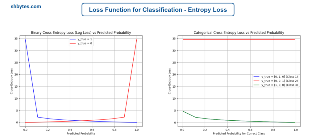
Example Program – Binary Cross-Entropy Loss
import numpy as np

# Binary Cross-Entropy Loss function
def binary_cross_entropy(y_true, y_pred):
    epsilon = 1e-15
    y_pred = np.clip(y_pred, epsilon, 1 - epsilon)  # Avoid log(0)

    # Compute Binary Cross-Entropy Loss
    loss = - (y_true * np.log(y_pred) + (1 - y_true) * np.log(1 - y_pred))
    return loss

# Generate a range of predicted probabilities from 0 to 1
predicted_probs = np.linspace(0, 1, 10)

# Calculate Binary Cross-Entropy Loss for y_true = 1 and y_true = 0
loss_true_1 = binary_cross_entropy(1, predicted_probs)
loss_true_0 = binary_cross_entropy(0, predicted_probs)

print(f"Binary Cross-Entropy Loss for true_1, {loss_true_1}")
print(f"Binary Cross-Entropy Loss for true_0, {loss_true_0}")

# Output
# Binary Cross-Entropy Loss for true_1, [3.45387764e+01 2.19722458e+00 1.50407740e+00 1.09861229e+00
#  8.10930216e-01 5.87786665e-01 4.05465108e-01 2.51314428e-01
#  1.17783036e-01 9.99200722e-16]
# Binary Cross-Entropy Loss for true_0, [9.99200722e-16 1.17783036e-01 2.51314428e-01 4.05465108e-01
#  5.87786665e-01 8.10930216e-01 1.09861229e+00 1.50407740e+00
#  2.19722458e+00 3.45395760e+01]
Example Program – Categorical Cross-Entropy Loss
import numpy as np

# Categorical Cross-Entropy Loss function
def categorical_cross_entropy(y_true, y_pred):
    epsilon = 1e-15
    y_pred = np.clip(y_pred, epsilon, 1 - epsilon)  # Avoid log(0)
    loss = - np.sum(y_true * np.log(y_pred), axis=1)
    return loss

# Generate a range of predicted probabilities for 3 classes
# For simplicity, we assume y_true is a one-hot vector for class 1 (e.g., [0, 1, 0])
classes = 3
predicted_probs = np.linspace(0.01, 0.99, 10)  # Range for predicted probabilities

# Create y_true as one-hot encoded vectors for each class
y_true_class_1 = np.array([[0, 1, 0]] * 10)  # One-hot for class 1
y_true_class_2 = np.array([[0, 0, 1]] * 10)  # One-hot for class 2
y_true_class_3 = np.array([[1, 0, 0]] * 10)  # One-hot for class 3

# For each class, we create predicted probabilities where the sum across each row is 1
y_pred_class_1 = np.column_stack([1 - predicted_probs, predicted_probs, np.zeros(10)])  # Class 1 is correct
y_pred_class_2 = np.column_stack([predicted_probs, 2 - predicted_probs, np.zeros(10)])  # Class 2 is correct
y_pred_class_3 = np.column_stack([predicted_probs, np.zeros(10), 1 - predicted_probs])  # Class 3 is correct

# Calculate the Categorical Cross-Entropy Loss for each case
loss_class_1 = categorical_cross_entropy(y_true_class_1, y_pred_class_1)
loss_class_2 = categorical_cross_entropy(y_true_class_2, y_pred_class_2)
loss_class_3 = categorical_cross_entropy(y_true_class_3, y_pred_class_3)

print(f"Categorical Cross-Entropy Loss for loss_class_1, {loss_class_1}")
print(f"Categorical Cross-Entropy Loss for loss_class_2, {loss_class_2}")
print(f"Categorical Cross-Entropy Loss for loss_class_3, {loss_class_3}")

# Output
# Categorical Cross-Entropy Loss for loss_class_1, [4.60517019 2.12956593 1.47938478 1.08866196 0.80843334 0.58978867
#  0.41047765 0.25848292 0.12657154 0.01005034]
# Categorical Cross-Entropy Loss for loss_class_2, [34.53877639 34.53877639 34.53877639 34.53877639 34.53877639 34.53877639
#  34.53877639 34.53877639 34.53877639 34.53877639]
# Categorical Cross-Entropy Loss for loss_class_3, [4.60517019 2.12956593 1.47938478 1.08866196 0.80843334 0.58978867
#  0.41047765 0.25848292 0.12657154 0.01005034]
Hinge Loss
The Hinge Loss is used for Support Vector Machines (SVM) and is designed for binary classification tasks. It penalizes predictions that are not only incorrect but also confidently incorrect.
Hinge Loss = $\sum_{i=1}^{N}\text{max}\left(0, 1 – y_{i}\cdot \hat{y}_{i} \right)$
Where, $y_{i}$ is the true label for the $i$-th sample, where $y_{i}$ ∈ {−1,1} and $\hat{y}_{i}$ is the predicted score (not a probability).
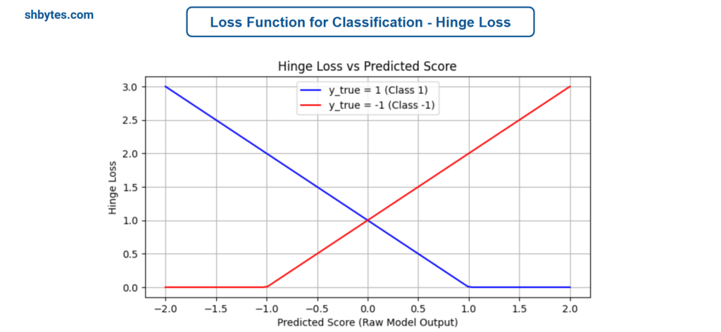
Example Program – Hinge Loss
import numpy as np
# Hinge Loss function
def hinge_loss(y_true, y_pred):
# Ensure y_true is either -1 or 1
loss = np.maximum(0, 1 - y_true * y_pred)
return loss
# Generate a range of predicted scores (raw model outputs) from -2 to 2
predicted_scores = np.linspace(-2, 2, 100)
# True labels for binary classification (-1 or 1)
y_true_class_1 = np.array([1] * 100) # True label for class 1
y_true_class_2 = np.array([-1] * 100) # True label for class -1
# Calculate Hinge Loss for both classes (Class 1 and Class -1)
loss_class_1 = hinge_loss(y_true_class_1, predicted_scores)
loss_class_2 = hinge_loss(y_true_class_2, predicted_scores)
print(f"Hinge Loss for loss_class_1, {loss_class_1}")
print(f"Hinge Loss for loss_class_2, {loss_class_2}")
# Output
# Hinge Loss for loss_class_1, [3. 2.95959596 2.91919192 2.87878788 2.83838384 2.7979798
# 2.75757576 2.71717172 2.67676768 2.63636364 2.5959596 2.55555556
# 2.51515152 2.47474747 2.43434343 2.39393939 2.35353535 2.31313131
# 2.27272727 2.23232323 2.19191919 2.15151515 2.11111111 2.07070707
# 2.03030303 1.98989899 1.94949495 1.90909091 1.86868687 1.82828283
# 1.78787879 1.74747475 1.70707071 1.66666667 1.62626263 1.58585859
# 1.54545455 1.50505051 1.46464646 1.42424242 1.38383838 1.34343434
# 1.3030303 1.26262626 1.22222222 1.18181818 1.14141414 1.1010101
# 1.06060606 1.02020202 0.97979798 0.93939394 0.8989899 0.85858586
# 0.81818182 0.77777778 0.73737374 0.6969697 0.65656566 0.61616162
# 0.57575758 0.53535354 0.49494949 0.45454545 0.41414141 0.37373737
# 0.33333333 0.29292929 0.25252525 0.21212121 0.17171717 0.13131313
# 0.09090909 0.05050505 0.01010101 0. 0. 0.
# 0. 0. 0. 0. 0. 0.
# 0. 0. 0. 0. 0. 0.
# 0. 0. 0. 0. 0. 0.
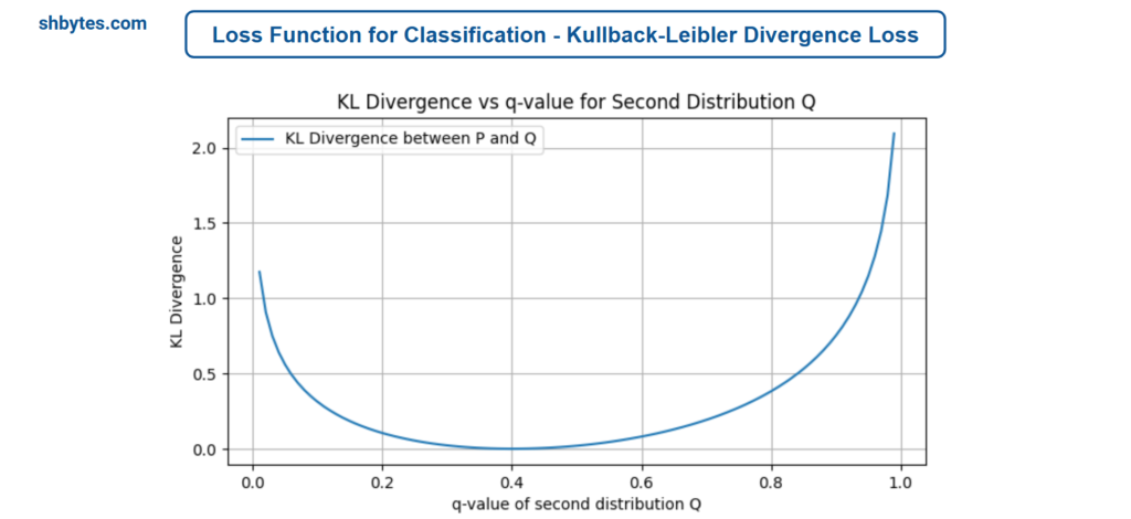
# 0. 0. 0. 0. ]Kullback-Leibler Divergence (KL Divergence)
Kullback-Leibler Divergence (KL Divergence) is used to measure the difference between two probability distributions: the true distribution P and the predicted distribution Q. This loss is particularly useful for generative models or when comparing distributions.
$D_{KL}\left(P\parallel Q \right) = \sum_{i=1}^{N}p\left(x_{i}\right)\text{log}\frac{p\left(x_{i}\right)}{q\left(x_{i}\right)}$
Where, $p\left(x_{i}\right)$ is the true probability distribution, $q\left(x_{i}\right)$ is the predicted probability distribution and logarithm is usually taken in base 2 for bits (in information theory) or base e for natural algorithms.
Example Program – Kullback-Leibler Divergence (KL Divergence) Loss
import numpy as np

# Function to calculate Kullback-Leibler (KL) Divergence
def kl_divergence(p, q):
    # Clip q values to avoid division by zero and log(0)
    epsilon = 1e-10
    q = np.clip(q, epsilon, 1.0)

    # Calculate the KL Divergence: sum(P * log(P / Q))
    return np.sum(p * np.log(p / q))

# Example usage:
# True distribution P and predicted distribution Q
# Both distributions should sum to 1 (valid probability distributions)

p = np.array([0.4, 0.6])  # True distribution
q = np.array([0.5, 0.5])  # Predicted distribution

# Calculate KL Divergence
kl_div = kl_divergence(p, q)
print(f"KL Divergence between P and Q: {kl_div}")

# To visualize KL Divergence for different distributions, we can plot it
# Generate different probability distributions for Q
q_values = np.linspace(0.01, 0.99, 100)
kl_values = []

# Calculate KL Divergence for different values of q (second distribution)
for q_val in q_values:
    q = np.array([q_val, 1 - q_val])  # q is [q_val, 1 - q_val]
    kl_values.append(kl_divergence(p, q))

# Output => KL Divergence between P and Q: 0.020135513550688863
Conclusion
In this article we learned about Loss Functions in Machine Learning. We learned about different type of loss functions like loss functions for regression, loss functions of classification and loss functions for specialized tasks. Which loss function you use depends on the problem you are trying to solve. For classification, Cross-Entropy Loss and Hinge Loss are the most commonly used, but specialized tasks like metric learning-e.g., Contrastive Loss or Triplet Loss-and generative modeling-e.g., KL Divergence-involve customized loss functions that handle unique requirements. The choice of an appropriate loss function guides the model to learn the right patterns and optimize the desired outcomes effectively.
ML code snippets and programs related to Loss Functions in Machine Learning, can be accessed from GitHub Repository. This GitHub repository all contains programs related to other articles in Machine Learning.
Related Topics
- What is Tokenization in NLP – Complete Tutorial (with Programs)What is Tokenization Tokenization is one of the major technique in Natural Language Processing (NLP) preprocessing that basically converts raw text into smaller, structured and organized units called tokens. These tokens can be words, subwords, sentences, or even characters. The size of tokens would depend on what form of processing is in view. Why Tokenization Matters in NLP Tokenization is important because Natural Language Processing (NLP) models cannot process texts without breaking it down into some form…
- What are Large Language Models (LLMs)Large Language Models (LLMs) have become the new paradigm for interacting with technology in NLP-based applications. LLMs are taking the center stage in both understanding and generating human language, ranging from conversational chat-bots to graphics generation systems. This article covers what exactly LLMs are, focusing on their main attributes and importance in NLP. What are…
- What are N-Gram Models – Language ModelsN-Gram Models N-Gram models are a fundamental type of language model in Natural Language Processing (NLP). These models predict the probability of a sequence of words with regard to the previous word in a fixed window, referred to as “n.” These models have been used in simpler language-related tasks and provide the foundation for more…
- Recurrent Neural Networks (RNNs) – Language ModelsWhat are RNNs (Recurrent Neural Networks) Recurrent Neural Networks, or RNNs, are variants of artificial neural networks. They have been designed for processing sequential data. Other than the conventional feed-forward neural networks, the connections in RNNs loop backward to themselves, which allows it to create and maintain memory of past inputs. This property makes RNNs…
- Natural Language Processing (NLP) – Comprehensive GuideNatural Language Processing (NLP) is a technology in the artificial intelligence domain that involves interaction between human communication and machines understanding. It empowers machines to process human languages in a meaningful and useful way. It enables machines to learn & understand human languages and become capable to generate meaningful output. This makes it possible for…
Excellent postings Cheers!
Good write ups. Thank you!